Now Reading: Supervised Machine Learning in a Nutshell for Ultimate Beginners
- 01
Supervised Machine Learning in a Nutshell for Ultimate Beginners

Supervised Machine Learning in a Nutshell for Ultimate Beginners
Table of Contents
Introduction to Supervised Learning
Supervised learning is one of the fundamental concepts in the field of machine learning, where a model learns from labeled data to make predictions or classifications.
But, what do we mean with labeled data?
Let’s assume we have ten images, and each of them features either a beer bottle or a wine bottle. At first, our first machine, which we will call Machine A, doesn’t know which bottles are for beer or wine. This information needs to be provided. We tell Machine A, “Look, the bottle in the first image is a beer bottle; the second one is a wine bottle; the third one is also a wine bottle. However, the bottle in the fourth image is a beer bottle,” and it will go on like that. This is called “labeling”; we label all the images according to which class they belong to.
Let’s check another example for our second machine, which is Machine B. Suppose we have hundreds of patient files, and each file has data about a patient. That data may include age, ethnicity, prescribed medications, hospital admissions if any, and previous diagnoses, etc. (these pieces of data are also called ‘features’). Then, we label those files, saying, “The patient in the first file is diabetic. The second one is healthy in terms of diabetes,” and so on.
Afterwards, our machines learn the underlying patterns between the features and the classes, which are diabetic and healthy, or beer bottle and wine bottle in our examples. From that point forward, when we give a new image to Machine A, it will be able to predict the bottle type in the image. If we pass a patient’s file to machine B, it will also predict whether the patient is diabetic or healthy. As you would expect, Machine A is trained on bottle images and cannot make predictions over patient files. Similarly, Machine B has the ability to make predictions for only patient files, and it will be speechless when faced with pictures of bottles.
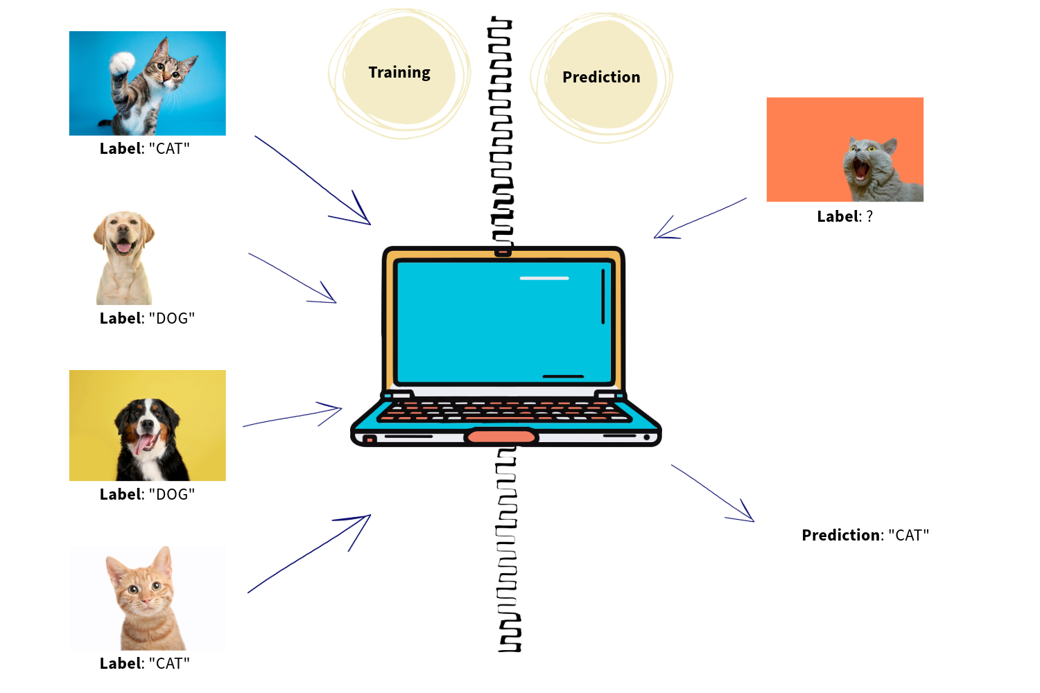
As it turns out, our machines were able to learn the relationships between features and classes under our supervision, thanks to our efforts for labeling the data. We treated them as if we were teachers. That is why we call this technique supervised learning.
Types of Supervised Machine Learning
Classification
As you may have noticed from the examples above, the predictions the machines made were to assign the inputs to a category or a class. The images were either beer bottles or wine bottles; a third type of bottle was not among the answers we expected from Machine A. Similarly, the answer we expected from Machine B was that the file owner was either diabetic or healthy in terms of diabetes; there was no third possibility.
This type of supervised learning is referred to as classification. The content of the machine’s predictions consists of predetermined classes, since they were trained to make predictions only in terms of these categories.
Regression
What about if we want our Machine C to predict a continuous number instead of a categorical distinct value?
Let’s say we have a real estate dataset including thousands of properties. Each property in this dataset has features such as address, number of bedrooms, surface area, garden existence, number of floors, age of building, etc. We tell Machine C that the first house’s selling price is $125k, the second’s is $329k, and so on. What we do here is to label all the properties with their selling prices. As you would guess, the selling price may be anything, any decimal number starting from 0. It is not possible to categorize all the decimal numbers, since they are infinite. In this case, first, Machine C will do a regression analysis, and then when we request it to predict a new property’s selling price, it will respond with a decimal number, which may not be among our initial labels.
This type of supervised learning is referred to as regression.
Common Algorithms Used for Supervised Learning
There are numerous algorithms being used to develop supervised machine learning models. While some of those are effective on small datasets, some may need larger ones to avoid the risk of overfitting. While some cannot handle missing data, some can overcome this. Each algorithm has its own advantages and disadvantages. That is why, prior to developing a machine learning model, it is important to contemplate what ideal algorithms can be used would be, considering the available data and the objectives.
In the table below, you will see some of the most common algorithms found in the literature.
| Algorithm | Description | For Which Dataset? | Pros | Cons | Learning Type |
|---|---|---|---|---|---|
| K-Nearest Neighbors (KNN) | Predicts labels based on the closest data points in feature space. | Small datasets with low noise. | Simple, no ‘actual’ training phase is required. | Slow for large datasets, sensitive to noise. | Classification, Regression |
| Decision Tree | Splits data into branches based on feature values to make predictions. | Structured datasets with clear splits. | Easy to interpret. Handles non-linear relationships. | Prone to overfitting on small datasets. | Classification, Regression |
| Random Forest | Ensemble of decision trees for improved accuracy and robustness. | Structured and noisy datasets. | Reduces overfitting compared to decision trees, works well with large datasets. | Computationally intensive for large forests. | Classification, Regression |
| Linear Regression | Models relationship between inputs and outputs with a linear equation. | Numeric and continuous data. | Simple, interpretable, and efficient. | Struggles with non-linear relationships. | Regression |
| Logistic Regression | Predicts probabilities for binary or multi-class classification problems. | Categorical and binary datasets. | Good for binary classification, interpretable. | Assumes linear separability. | Classification |
| Support Vector Machine (SVM) | Finds the best hyperplane to separate classes in high-dimensional space. | High-dimensional and small datasets. | Effective for high-dimensional data, robust to overfitting. | Sensitive to hyperparameter tuning. | Classification, Regression |
| Gradient Boosting | Combines weak learners iteratively to minimize errors. | Complex and noisy datasets. | High accuracy, handles non-linear data effectively. | Computationally expensive, prone to overfitting. | Classification, Regression |
| Naive Bayes | Based on Bayes’ theorem, assumes independence between features. | Text and categorical data. | Fast, works well for text classification. | Assumption of independence rarely holds. | Classification |
How to Evaluate Performance of Supervised Machine Learning Models
Since machine learning is not a magic, its predictions sometimes will be wrong while sometimes correct. Therefore, after we train our model with an algorithm from the listed ones above, we would like to see how good the model’s predictions are. We may need to take various actions if the performance is not sufficient, such as changing the algorithm we used for training, hyperparameter tuning, re-exploring the data, conducting different data transformations than we did before, producing synthetic data, searching for extra real data, etc. Actions are countless.
Performance measurement metrics change depending on whether the supervised learning type is classification or regression.
Classification Evaluation Metrics
Accuracy: Accuracy measures the percentage of correctly classified samples out of the total samples. Let’s say Machine A makes predictions for 100 images to assign each of them to a category. If 72 predictions are correct out of those 100, then the accuracy is 72%. As you see, it is very straightforward to interpret. However, it may not be reliable for imbalanced datasets.
Accuracy = \frac {TP + TN} {All\>Instances}
Precision: Precision quantifies how many of the predicted positive instances are correct. Let’s say our positive instance is a cat, not a dog. Precision answers this question: What percentage of the pictures Machine A assumed were ‘cats’ were actually cats?
Precision = \frac {TP} {TP + FP}
Recall (Sensitivity): Recall measures how many actual positives are identified. Recall answers this question: What percentage of the images that actually contained cats could Machine A predict as ‘cat’?
Sensitivity = \frac {TP} {TP + FN}
F1 Score: The F1 Score is the harmonic mean of precision and recall, offering a balanced metric for imbalanced datasets.
F1\>Score = 2 * \frac {(Precision*Recall)} {(Precision+Recall)}
Confusion Matrix: All the metrics above can be seen on a confusion matrix easily. A confusion matrix is nothing more than a simple table in which we place facts and predictions according to their truth or falsity. A simple example is shown below.
| Realities & Predictions | Actual Cat (Positive) | Actual Dog (Negative) |
| Predicted Cat (Positive) | 48 (True Positive — TP) | 3 (False Positive — FP) |
| Predicted Dog (Negative) | 2 (False Negative — FN) | 47 (True Negative — TN) |
ROC-AUC: The Receiver Operating Characteristic Curve — Area Under the Curve (ROC-AUC) measures the ability of the classifier to distinguish between classes. AUC values range from 0 to 1, with higher values indicating better model performance.
You can read exciting story of evaluation metrics of classification models here: The Metric Chronicles: Mighty Guardians of the Classification Realm
Regression Evaluation Metrics
Mean Squared Error (MSE): This metric calculates the average squared difference between the predicted and actual values. It heavily penalizes larger errors, making it sensitive to outliers.
MSE = \frac {\displaystyle\sum_{i=1}^n (y_{i} - p_{i})^2} {n}
— where y_{i} is the true (actual) value, while p_{i} is the corresponding predicted value. We then square all the differences between the real and predicted values and add them all up. Then we divide the sum of squares by the total number of instances.
Mean Absolute Error (MAE): MAE computes the average of absolute differences between predictions and actual values. It provides a straightforward measure of prediction accuracy and is less sensitive to outliers compared to MSE.
MAE = \frac {\displaystyle\sum_{i=1}^n \left|y_{i} - p_{i}\right|} {n}
You will notice that large differences are less penalized than MSE because we do not square the differences between the actual and predicted values.
R-squared: R-squared indicates the proportion of the variance in the dependent variable that is predictable from the independent variables. A higher R-squared value signifies better model performance in capturing data variability.
R^2 = 1 - \frac {\displaystyle\sum_{i=1}^n (y_{i} - p_{i})^2} {\displaystyle\sum_{i=1}^n (y_{i} - m)^2}
— where y_{i} is the true (actual) value, while p_{i} is the corresponding predicted value, and m is the mean of the actual y_{i} values.
- If R^2 = 1, then the model fits to data perfectly and it explains all the variability. All the actual values are on the fitted data. All the predictions are totally true. No difference between actual and predicted values, not even 0.0000001.
- If R^2 = 0 the model does not explain any of the variability, and the predictions are no better than simply using the mean of the actual values.
- If R^2 < 0, the model is really bad, and simply using the mean for prediction is even better than the model itself.
- For an ideal model, we expect R^2 to be between 0 and 1, and closer to 1.
You can check the funny story of MAE, MSE and R-Squared here: When Metrics Collide: A Clash of Regression Titans in the Spotlight.
Conclusion
Supervised machine learning has been widely used across various industries for applications like spam detection, fraud prevention, or medical diagnosis. It serves as the backbone for many of today’s AI-driven applications. By utilizing labeled datasets, it facilitates precise predictions and decisions, making it invaluable in numerous fields. The need for extensive labeled datasets is one of the challenges, since it may need a lot of manual effort time to time. However, its effectiveness and adaptability make it a cornerstone of machine learning. Understanding its core principles and methods provides a solid foundation for exploring advanced techniques and applications.


Orcun Tasar
This post will be updated regularly.
Pingback: When Metrics Collide: A Clash of Regression Titans in the Spotlight - Longoz Park
Pingback: The Metric Chronicles: Mighty Guardians of the Classification Realm - Longoz Park